Simulating 3D Room Modes in the Browser: Implementing Voxel Finite-Difference Helmholtz Solvers in Python & WebGL

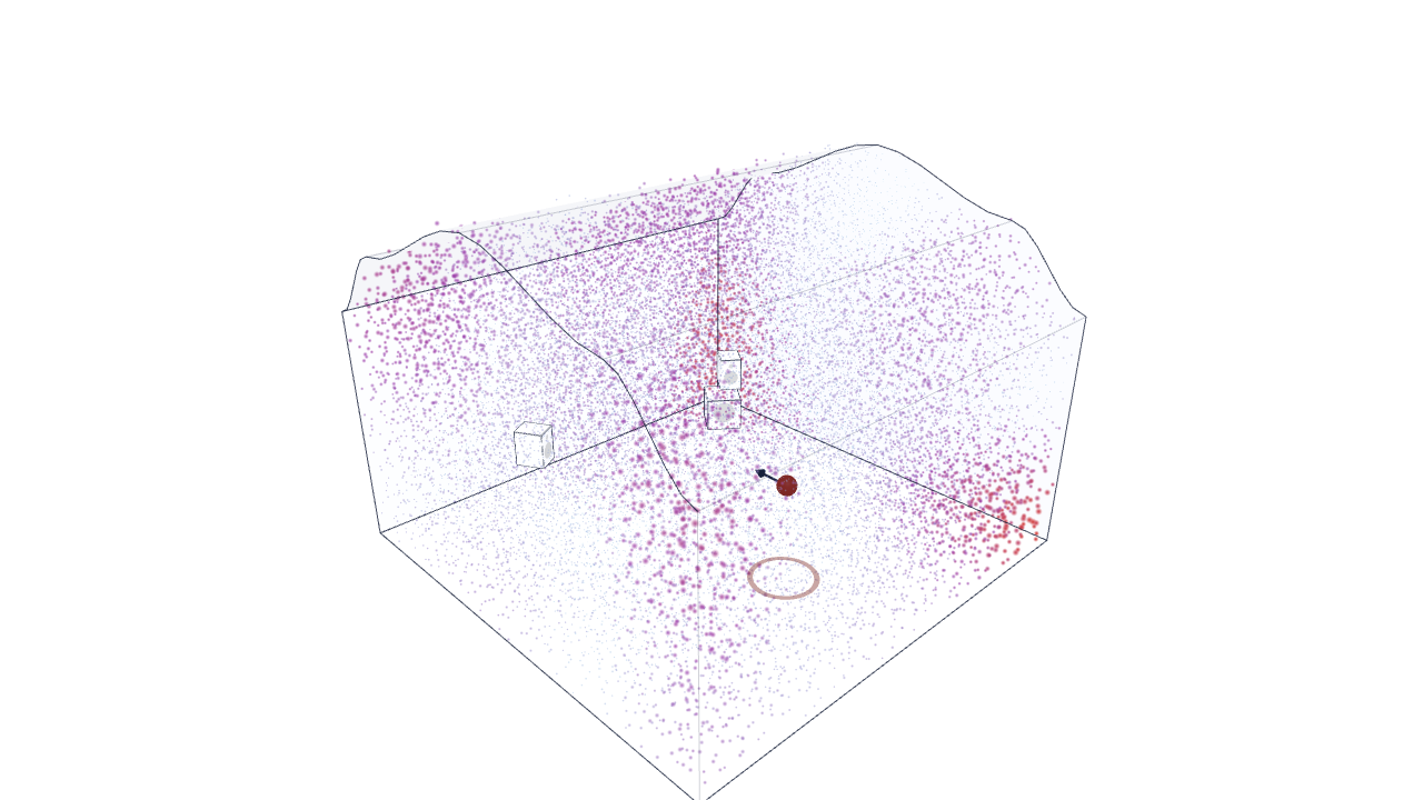
TL;DR: Ray tracing breaks down in small room acoustics below 200 Hz because sound behaves as discrete standing waves rather than geometric rays. We built roomtreatment.diy by discretizing arbitrary 3D room geometries into a uniform voxel grid ($h = 0.18\text{ m}$ pitch), solving the spatial negative Laplacian $-\nabla^2$ via SciPy's sparse Lanczos eigensolver (scipy.sparse.linalg.eigsh), and applying first-order acoustic perturbation theory to predict modal RT60 decay and speaker/listener nulls in seconds directly on the web.

Most web-based audio tools treat room acoustics like optics. They draw straight lines from a speaker to a wall, bounce them off at equal angles, and call it a day.

That works fine for high frequencies. But below 200 Hz, ray tracing is a lie.

In a typical home studio or listening room, a 50 Hz sound wave is nearly 7 meters long. It doesn't bounce around like a laser beam. It fills the room, wraps around itself, and creates massive acoustic standing waves—room modes. You get localized peaks where bass booms uncontrollably and deep nulls where low frequencies vanish entirely.

If you want to simulate how bass actually behaves in real, non-shoebox rooms (L-shapes, slanted ceilings, alcoves), you have to solve the 3D wave equation directly. Here is how we implemented a full spatial Finite-Difference Helmholtz eigensolver for the web using Python, SciPy, and WebGL.

The Physical Model: Helmholtz Equation & Boundary Conditions

In the low-frequency domain ($f < 200\text{ Hz}$), acoustic sound pressure $p(\mathbf{r}, \omega)$ inside a room volume $\Omega$ satisfies the inhomogeneous Helmholtz equation:

$\nabla^2 p(\mathbf{r}) + k^2 p(\mathbf{r}) = -i \omega \rho_0 q(\mathbf{r})$

where $k = \frac{2\pi f}{c}$ is the wavenumber, $c = 343\text{ m/s}$ is the speed of sound in air, and $\rho_0 = 1.204\text{ kg/m}^3$ is air density.

At room boundaries (rigid drywall, concrete, or glass), sound waves reflect almost completely. This means the normal particle velocity at the boundary face is zero. Mathematically, we impose homogeneous Neumann boundary conditions:

$\frac{\partial p(\mathbf{r})}{\partial n} = 0 \quad \text{on } \partial \Omega$

where $n$ is the unit normal vector pointing out of the room surface.

Step 1: Voxelizing Arbitrary 3D Geometries

Shoebox analytical equations ($f_{n_x, n_y, n_z} = \frac{c}{2}\sqrt{(n_x/L_x)^2 + (n_y/L_y)^2 + (n_z/L_z)^2}$) break down the moment a room has an L-extension, a dormer window, or an angled wall.

To support real-world room shapes, we discretize the 3D domain into a uniform voxel grid with a spatial step $h = 0.18\text{ m}$.

import numpy as np
from scipy.sparse import csr_matrix

def build_voxel_laplacian(air_voxels_mask, h=0.18):
    """
    Constructs the 7-point negative finite-difference Laplacian matrix 
    with Neumann boundary conditions on arbitrary interior air voxels.
    """
    # Map (x, y, z) 3D grid index to a continuous 1D index
    grid_shape = air_voxels_mask.shape
    air_indices = np.argwhere(air_voxels_mask)
    voxel_to_idx = {tuple(coord): i for i, coord in enumerate(air_indices)}
    num_air = len(air_indices)
    
    row_ind, col_ind, data = [], [], []
    
    # 6 cardinal neighbor direction vectors
    neighbors = [(-1,0,0), (1,0,0), (0,-1,0), (0,1,0), (0,0,-1), (0,0,1)]
    
    for i, (x, y, z) in enumerate(air_indices):
        active_neighbors = 0
        for dx, dy, dz in neighbors:
            neighbor_coord = (x + dx, y + dy, z + dz)
            if neighbor_coord in voxel_to_idx:
                active_neighbors += 1
                j = voxel_to_idx[neighbor_coord]
                # Off-diagonal element for interior coupling
                row_ind.append(i)
                col_ind.append(j)
                data.append(-1.0 / (h**2))
        
        # Diagonal element enforces Neumann boundary implicitly
        # (ghost cell values equal boundary cell values)
        row_ind.append(i)
        col_ind.append(i)
        data.append(active_neighbors / (h**2))
        
    L = csr_matrix((data, (row_ind, col_ind)), shape=(num_air, num_air))
    return L, air_indices

By adjusting the diagonal term to match the exact number of active interior neighbors ($N_{\text{adj}} \le 6$), Neumann zero-flux boundary conditions are enforced naturally without constructing explicit ghost cells outside the mesh.

The resulting Laplacian matrix $\mathbf{L}$ is sparse, real, symmetric, and positive semi-definite.

Step 2: Extracting Mode Shapes with Shift-and-Invert Lanczos

We don't need all 50,000 eigenvalues of the grid. We only care about the lowest $M \approx 50\text{ to } 100$ acoustic natural frequencies below $200\text{ Hz}$.

Using SciPy's interface to ARPACK (scipy.sparse.linalg.eigsh), we execute a Shift-and-Invert Arnoldi/Lanczos iteration targeted near spectral shift $\sigma \approx 0$:

from scipy.sparse.linalg import eigsh

def eigensolve_room_modes(L, num_modes=60, c=343.0):
    """
    Solves L * phi = lambda * phi for the lowest spatial modes.
    Returns natural frequencies (Hz) and mode shape vectors.
    """
    # Shift-and-invert spectral transformation around sigma = 1e-5
    eigenvalues, eigenvectors = eigsh(
        L, 
        k=num_modes, 
        which='SM', 
        sigma=1e-5
    )
    
    # Convert spatial Laplacian eigenvalues (k^2) to frequency (Hz)
    # lambda = k^2 = (2 * pi * f / c)^2  ==>  f = (sqrt(lambda) * c) / (2 * pi)
    k_vals = np.sqrt(np.maximum(eigenvalues, 0))
    freqs_hz = (k_vals * c) / (2.0 * np.pi)
    
    return freqs_hz, eigenvectors

Each column of eigenvectors represents an unperturbed 3D mode shape $\phi_m(\mathbf{r})$. We normalize these vectors against the total room volume $V$:

$\frac{1}{N_{\text{AIR}}} \sum_{i=1}^{N_{\text{AIR}}} \phi_m^2(i) = 1$

Step 3: First-Order Acoustic Perturbation for Absorbing Panels

What happens when a user drops a $50\text{ mm}$ thick porous absorber onto a side wall? Re-running eigsh for every single panel move would take seconds and destroy real-time UI responsiveness.

Instead, we use First-Order Acoustic Modal Perturbation Theory.

A panel covering surface area $S_p$ with real acoustic admittance $\text{Re}(Y_p) \approx \frac{\alpha_p}{4}$ dissipates energy from mode $m$ proportional to the sound pressure square at that specific wall surface:

$d_{\text{diss}, m}^{(p)} = \text{Re}(Y_p(f_m)) \cdot \frac{c \cdot h^2}{V} \sum_{k \in \text{panel\_surface\_voxels}} \phi_m^2(k)$

The updated quality factor $Q_m$ and modal decay time $T_{60, m}$ are computed instantly:

$\eta_m^{\text{total}} = \eta_m^{\text{bare}} + \frac{1}{2 k_m} \sum_{p \in \text{placed\_panels}} d_{\text{diss}, m}^{(p)}$

$Q_m = \frac{1}{2 \eta_m^{\text{total}}}, \quad T_{60, m} = \frac{3.01 \cdot Q_m}{\pi f_m}$

This calculation takes less than 1 millisecond. The user slides a panel along the wall in the 3D canvas, and the low-frequency frequency response graph updates at 60 FPS.

Comparing Simulation Models across Regimes

Try the Interactive Simulation

We wrapped this entire solver pipeline into a fast, free WebGL interface at roomtreatment.diy. You can input your room dimensions, drag your speakers and listening desk around, and instantly inspect the 3D standing wave heatmaps and frequency response nulls for your exact space.

No installation required, no signup wall to run your first room calculation.

Hacker News Excerpt (Show HN)

Title: Show HN: roomtreatment.diy – Free web-based 3D room acoustics simulator

Post Body: Hey HN, I built roomtreatment.diy—a free web tool that simulates 3D room acoustics and standing waves.

Most web acoustic calculators use ray tracing or simple shoebox equations. But ray tracing completely breaks down in small rooms below 200 Hz, where sound acts as discrete standing waves rather than geometric rays.

To solve this for non-rectangular rooms (L-shapes, slanted ceilings), the backend discretizes the space into a 3D voxel grid ($h=0.18\text{ m}$ pitch) and solves the spatial negative Laplacian matrix $-\nabla^2$ under Neumann boundary conditions using SciPy's sparse Lanczos eigensolver (scipy.sparse.linalg.eigsh). When you place wall absorbers or corner bass traps, it uses 1st-order modal perturbation theory to recompute modal $T_{60}$ decay rates and listener nulls in under 1ms.

It's completely free, runs client-side interactive WebGL rendering, and requires no login to build a room model. I'd love your feedback on the physics model and UI experience!