Why Ray Tracing Fails Below 200 Hz: Hybrid Wave PDE and Geometrical Acoustics in Small Rooms

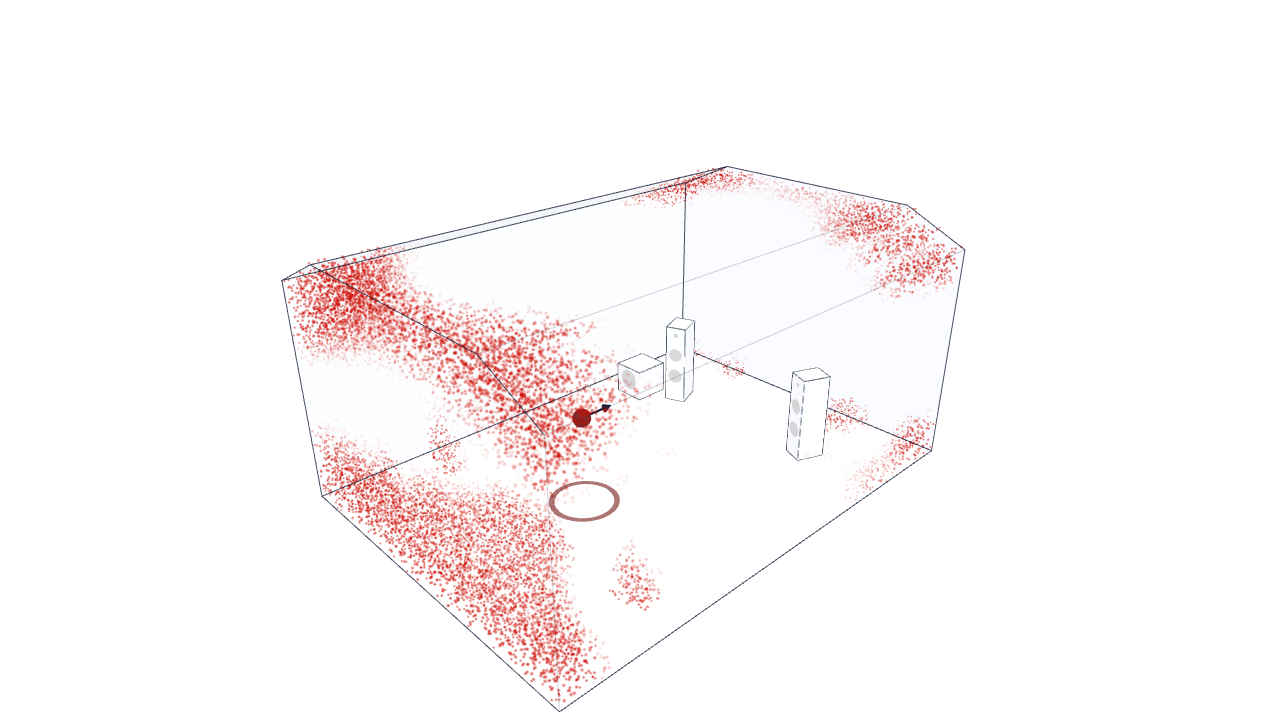
TL;DR: Ray tracing assumes sound propagates like light rays along straight vectors. In small enclosed spaces below the Schroeder cutoff frequency ($f_s \approx 2000 \sqrt{T_{60} / V}$), acoustic wavelengths exceed boundary dimensions, turning the sound field into discrete wave interference. Here is why room acoustics simulators like roomtreatment.diy use a hybrid architecture: Finite-Difference wave PDEs for bass frequencies and Image Source ray tracing for mid-to-high specular reflections.

If you've ever used acoustic modeling software, you've seen ray tracing. Tens of thousands of virtual sound rays shoot out from a speaker vector, reflect off walls like billiard balls, and land in a listener's ears.

It looks impressive. The 3D render is clean. The math feels intuitive.

And below 200 Hz, it is almost completely wrong.

Understanding why ray tracing breaks down in small room acoustics isn't just an academic exercise. It dictates whether your studio monitor placement fixes a 15 dB bass drop at 60 Hz or accidentally makes it worse.

The Physics Bottleneck: Ray Optics vs. Wave Mechanics

Ray tracing operates under geometric acoustics. It makes a fundamental physical assumption: the wavelength of sound $\lambda$ is infinitely small compared to the dimensions of the room and the boundaries it hits.

At 4,000 Hz, sound waves are less than 9 centimeters long. A $4\text{ m} \times 5\text{ m}$ wall looks like a massive specular mirror. Sound strikes it and bounces at an angle equal to its incident angle. Geometric rays work beautifully here.

Now drop down to 45 Hz. The wavelength of a 45 Hz tone is 7.6 meters.

That wavelength is larger than the height of your ceiling. The sound wave doesn't "hit" the front wall and reflect off like a flashlight beam. The wave occupies the entire room simultaneously. It wraps around boundaries, diffracts around desk corners, and collides with its own reflection to set up localized, stationary pressure zones.

This frequency boundary isn't arbitrary. It is defined by the Schroeder Cutoff Frequency ($f_s$):

$f_s \approx 2000 \sqrt{\frac{T_{60}}{V}}$

For a typical $45\text{ m}^3$ home studio with a target reverberation time $T_{60} = 0.35\text{ seconds}$, the Schroeder cutoff sits right around 175 Hz to 200 Hz.

The 200 Hz Schroeder cutoff splits the audible range (20 Hz – 4,000 Hz+) into two regimes with fundamentally different physics:

What Happens When You Ray-Trace Bass?

If you try to compute low-frequency response using ray tracing, three major errors occur:

1. Zero Phase Interference: Rays track energy intensity, not complex acoustic phase ($\mathbf{p} = |P|e^{i\phi}$). Ray tracing cannot naturally model two out-of-phase bass waves arriving at a chair and canceling each other out to create a 20 dB notch.
2. Missing Boundary Admittance: Porous absorbers work on particle velocity near rigid surfaces. Ray tracing treats absorption as a flat scalar percentage ($\alpha = 0.70$), ignoring how acoustic impedance changes with wave incident angle and modal velocity nodes.
3. Artificial Spatial Smoothing: Ray tracing averages energy over spatial bins. In real rooms, moving your listening chair just 30 centimeters forward can shift you out of a 70 Hz modal null into a high-pressure zone. Ray tracing smoothes this sharp gradient away.

The Solution: A Hybrid Simulation Pipeline

To get accurate predictions without sending compute time into hours, roomtreatment.diy uses a hybrid physical solver pipeline.

Below $200\text{ Hz}$, we treat the air inside the room as a continuous pressure field, solving the discretized 3D Helmholtz PDE:

$\nabla^2 p(\mathbf{r}) + k^2 p(\mathbf{r}) = 0$

We run a 3D Voxel Finite-Difference stencil ($h = 0.18\text{ m}$) coupled with SciPy's sparse Lanczos solver (scipy.sparse.linalg.eigsh). This extracts the exact spatial mode shapes $\phi_m(\mathbf{r})$ and standing wave pressure nodes across the floorplan.

Above $200\text{ Hz}$, modal density explodes to dozens of overlapping modes per Hertz. Here, wave PDEs are unnecessary and computationally wasteful. We switch to the Image Source Method (ISM) for early specular mirror points ($t < 15\text{ ms}$) combined with stochastic ray tracing for high-frequency RT60 energy decay.

The hybrid pipeline:

1. Input: room shape, speaker positions, panel placements.
2. Split by frequency:
   • Below 200 Hz — Modal Wave PDE Solver: 7-point voxel Laplacian, Lanczos sparse eigensolver, 1st-order perturbation.
   • Above 200 Hz — Ray Tracing & ISM Solver: mirror image sources (ISM), 10,000 stochastic rays, Schroeder decay integration.
3. Output: combined full-spectrum response, 20 Hz – 20 kHz.

Simulators vs. Rules of Thumb: A Performance Comparison

Test Your Room Geometry

You don't need a PhD in computational acoustics to see how standing waves behave in your space. We exposed our hybrid wave PDE and ray-tracing solver engine in a clean, interactive browser app at roomtreatment.diy.

Set your room dimensions, position your speakers, and inspect the real low-end modal peaks and high-end reflection points in under 5 seconds.